Lagrange Multipliers – A Historical Approach? – Teaching Mathematics: What, When and Why

September 1, 2023

Lagrange Multipliers – A Historical Approach?

In the site Bad Mathematics, Marty and Christian R have recently been discussing the relation between History and Mathematics. Their discussion was wide ranging but the pointy end of it seems to be whether maths teaching benefits from presenting a topic in its historical context. Such an approach may offer a natural introduction, motivating the topic and leading directly to applications. The alternative is to offer the modern pared-down version, direct and logical. At the same time I was preparing this post which relates my personal experience of a lecture that offers evidence for both sides. The topic was Lagrange multipliers, so let me start with a quick introduction for newbies.

Suppose we wish to find the minimum value for the function $f(x) = x^2+y^2$ but are restricting the search to where $2x+y=5$ , “constrained optimization”. One method that used to be taught in schools is to solve the constraint for one of the variables, say $y=5-2x$ , and then substitute this into the function, giving $f(x) = x^2 + (5-2x)^2$ . It’s now a function of a single variable so let’s use calculus to find the turning point. [Overkill here as the function is a quadratic.] $f'(x) = 2x-4(5-2x) = 0$ so $x=2, y=1$ giving a minimum of $5$ .

The Lagrange method instead considers a combination of the objective and the constraint, $F(x,y,\lambda) = x^2+y^2 +\lambda (2x+y-5)$ . Here, instead of reducing the variables to just one, we have increased them to three by adding this mysterious variable $\lambda$ , called the Lagrange multiplier. Now we compute the partial derivatives $\frac{\partial F}{\partial x}$ , $\frac{\partial F}{\partial y}$ and $\frac{\partial F}{\partial \lambda}$ , equate them to $0$ , giving 3 equations for 3 unknowns: $\,2x+2\lambda=0$ , $\,2y+\lambda=0$ and $\,2x+y-5=0$ . These show again that $x=2$ , $y=1$ , and for what it is worth, $\lambda=-2$ .

Why make things harder in this way? Well in many cases the constraint equation cannot be solved to get one variable in terms of the other. For example, what if the constraint is $e^{xy} +y=x$ ? The Lagrange multiplier method will still work, at least it will give a system of 3 simultaneous equations that can be solved numerically.

So how did my lecturer approach this? She started by defining “infinitesimals”. Yes! Back in the 60s, optimization research papers and textbooks were still using those critters that are infinitely small but not zero. But she must have realized they were problematic because she had a new definition. Instead of defining $dx$ to be infinitely small, it was just an ordinary non-zero number. Then for $y=f(x)$ she defined $dy$ to be $f'(x) dx$ . Then $f'(x)$ really is the fraction $\frac{dy}{dx}$ . To obtain a maximum for $f$ she just put $dy=0$ . Looking back now I see that she was effectively putting $f'(x)=o$ so maybe she was ahead of her time!

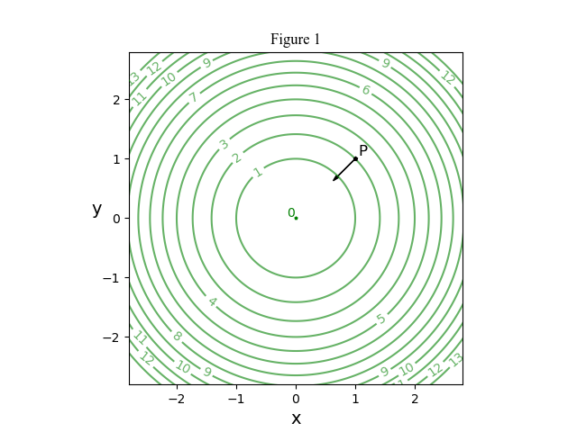
My lecturer then introduced the problem of optimizing $f(x,y)$ with constraint $g(x,y)=c$ . Magically the new function $F(x,y,\lambda)=f(x,y) +\lambda (g(x,y)-c)$ appeared and she proceeded to prove that it gave the same constrained optimum if we somehow put $dF=o$ . But my brain refused to follow the reasoning; I was still staring at that damned $\lambda$ . Where had it come from? The lecture might have been logically correct, but for me not psychologically correct.

Over the next few decades I would occasionally recall these Lagrange things, but never found the time to solve the mystery of their origin. Until 1999 that is, when I accepted a job in a research team at Monash, implementing optimization algorithms in a suite of software. Before starting I decided to resolve the mystery, just for self respect.

Lagrange and I shared the same handicap. We both learned calculus as a tool for modelling dynamics. We both missed out on the modern approach that divorces subjects from their roots. In Lagrange’s day the hot topic was the use of potential theory for dynamics. For example if a particle is moving under a scalar potential $f(x,y) = x^2 + y^2$ , the force acting on it is the vector $F=-\nabla f = -[\frac{\partial f}{\partial x}$ $, \frac{\partial f}{\partial y}] = [-2x, -2y]$ . In Figure 1 we see level curves for $f$ . At the point $P=(1,1)$ the force will be $[-2,-2]$ (shown not to scale) which will push the particle toward the origin. At the origin the force is zero, so the particle is in equilibrium there. The origin gives stable equilibrium which here corresponds to a minimum potential for $f$ .

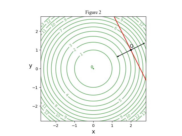
Now let’s introduce the constraint $g(x,y) = 2x+y-5=0$ . If the particle is constrained to that line then the new minimum potential is at the point $Q$ in Figure 2. How does that happen? To keep the particle on the line there must be a reaction force holding it there. But the particle is free to move along the line, so this force must be perpendicular to that line. Thus it will have the form $\lambda\,\nabla g(x,y)$ . But there is still the force $-\nabla f(x.y)$ due to the potential field. For minimum $f$ there is equilibrium; the two forces must exactly balance, $\lambda\,\nabla g(x,y) = -\nabla f(x,y)$ . Writing $F(x,y,\lambda) = f(x,y) + \lambda g(x,y)$ the minimizing point must satisfy $\frac{\partial F}{\partial x} =0$ and $\frac{\partial F}{\partial y} =0$ . That mysterious $\lambda$ is just a scale factor to give the correct reaction force.

Time for a literature search. Damn. Wikipedia gives almost an identical derivation to mine. So I pull down my 70s texts on optimization. None use this approach. One takes the lecturer’s route of plucking the Lagrange multiplier from nowhere. The others find different algebraic routes, none obvious. My conclusion is that Lagrange almost certainly used the dynamics argument but this was neglected when calculus was cleansed of physics.

How does this answer the issue of the historical approach to teaching mathematics?

Treating optimization as an exercise in Physics makes the derivation intuitive and easy. The historical approach is good.
Sticking to the traditional use of infinitesimals just muddies the issue for a modern reader. The historical approach is bad.

Furthermore

for those interested in the optimization theory …

A: What would it mean if we found $\lambda=o\;$ ?

B: We have been finding stationary points. Usually the nature of the optimization problem fingers the point as giving either a minimum or a maximum. If in doubt then one may resort to the Hessian matrix.

C: Suppose that we optimize $f(x_1, x_2, \ldots, x_n)$ with several constraints $g_i(x_1, x_2, \ldots, x_n)=0, \hbox{ for }i=1,2,\ldots ,m<n$ . Then for equilibrium, the force due to the potential function $-\nabla f$ must be balanced by a linear combination of reactions from the various constraints, $\sum_{i=1}^{i=m} \lambda_i\nabla g_i$ . This gives $F(x_1, x_2, \ldots, x_n, \lambda_1, \ldots, \lambda_m )$ equal to $f(x_1, x_2, \ldots, x_n + \sum_{i=1}^{i=m} \lambda_i\nabla g_i(x_1, x_2, \ldots, x_m)$ and all its derivatives zero. Here the force due to the potential is in the space spanned by the $\nabla g_i~$ ; a natural introduction to the more abstract linear algebra.

D: If a constraint is an inequality constraint, rather than an equality one, then if that constraint is active, the corresponding force vector has a specified sense. The Lagrange multiplier for that constraint will be either strictly positive or strictly negative, depending on the allowed direction of the inequality. We are on the road to Kurush-Kuhn-Tucker theory.

E: Returning to 2 dimensions and 1 constraint, an engineer may be interested in the trade-off between the constraint and the minimum $f\;$ . What is the “sensitivity” of the minimum to variations in that constraint? Figure 3 shows (in red) points allowed by the constraint $g(x,y)= 2x+y-c=0\;$ for various $c$ . As $c$ increases from $5$ , the corresponding optimal point moves outward from $Q$ and the minimal $f$ will increase. Keep in mind that $\nabla f$ gives the direction of maximal rate of change of $f$ and its magnitude is that rate of change. So if $s$ is displacement outward in the force direction, then $\frac{df}{ds} = |\nabla f|$ . Similarly $\frac{dc}{ds} = |\nabla c|$ . Hence $\frac{df}{ds} = -\lambda \frac{dc}{ds}$ , giving $\frac{df}{dc} = -\lambda\;$ . At the point $Q$ we saw that $\lambda = -2$ , so $\frac{df}{dc} = 2$ . So $\lambda$ measures the rate of trade-off between the constraint parameter $c$ and the optimal $f$ .

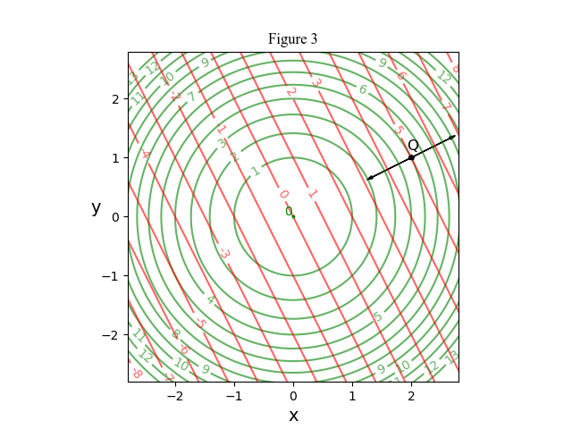
F: Looking again at Figure 3, suppose that we swap the roles of the families of contours. Now the green contours are the constraints and the red ones represent the function to be optimized. This time we obtain $F(x,y,\lambda) = 2x+y + \lambda(x^2+y^2-f)$ . For constraint $f=5$ the optimal point is again $Q$ giving $c=5$ although this time we have maximized $c$ . $\lambda$ will be $-1/2\;$ . This new problem is called the “dual” of the original.

G: Here is a classic pair of dual optimization problems. A nice exercise is to draw the relevant level curves.

A farmer is fencing a rectangular paddock on 3 sides. (The other side uses an existing fence.)

Suppose the new fence has length 800 m. Find the dimensions of the paddock that has maximum area.
Suppose instead that the enclosed area needs to be 80,000 m2. Find the dimensions of the paddock that will use minimum fence length.

H: The physical interpretation of Figure 3 is a gift that keeps giving. In that figure interpret the two contour families as competing objectives. This leads to a new direct search algorithm for bi-objective optimization.

EngOpt2012 Download

Uncategorized

Posted by:

tom

15 responses to “Lagrange Multipliers – A Historical Approach?”

Dr Mike

September 1, 2023 at 6:10 pm

Thanks for posting it, Tom. I like the historical approach. As you pointed out, it provides the context and motivation for a certain mathematical method. While writing my PhD [many years ago], I had articles from as far back as 19 century. My viva examiner grilled me out for that however defended the usage of such an ‘old’ bibliography with exactly the same words: context and motivation. Mathematics is the language and more than often use of the language without understanding its meaning less to problems.

LikeLike

Reply
tom

September 1, 2023 at 7:35 pm

Thanks Mike. I guess you have many examples where history provides a clear path for presentation of a topic. And I hope you will find time to present them on this site?
On the other hand, as Marty has found, the historical milieu of a new idea may be confused and confusing and it may take generations of work to make the idea clear. I would love people to present examples of this also.

LikeLike

Reply
1. Glen Wheeler
  
  September 2, 2023 at 1:03 am
  
  I think you have a good example here already: calculus. It would be quite insane to try to present calculus in a historically faithful way!
  
  LikeLike
  
  Reply
  1. tom
    
    September 3, 2023 at 9:25 am
    
    You are probably right on that topic. I say “probably” because I did with one student give her a first taste of calculus by “deriving” $A=\pi r^2$ using what the ancient Greeks “must” have done before settling on the method of exhaustion. This just broke the area of a disc into infinitely many circles. I don’t think she was damaged by the lesson, rather the opposite 😉
    
    LikeLike
2. Dr Mike
  
  September 3, 2023 at 2:13 am
  
  Hi Tom, no doubt we cannot always understand the rationale and motivation behind the mathematical assertion. We also always have a danger of drowning ourselves between Leibnitz and Newton instead of learning a modern explanation. However, the author’s motivation can more than often bring a light of clarity on this or the other mathematical statement. Why regression is called regression would definitely be a nice story with a historical background.
  
  LikeLike
  
  Reply
  1. tom
    
    September 3, 2023 at 9:20 am
    
    My guess is that it had to do with “regression to the mean”? But I have never seen any connection between that and fitting a straight line! Can you enlighten?
    
    LikeLike
Tom’s Posts Are (Lagrange) Multiplying – BAD MATHEMATICS

September 2, 2023 at 1:35 pm

[…] has a new post on his Teaching Mathematics blog: Lagrange Multipliers – A Historical Approach? Tom riffs off […]

LikeLike

Reply
Glen Wheeler

September 3, 2023 at 10:43 am

Hi Tom,

I couldn’t find the “reply” button under your reply… might be a mobile issue, or is it something deliberate?

On topic: IMO anything Ancient Greeks is not calculus. For the example you mention, I’m assuming you are talking about the scaling property. Is there evidence of Greeks using calculus-like reasoning?

I feel like it is a little bit difficult for beginners to “realise” that geometric notions like area and volume are functions of parameters (like radii and side lengths). They are taught for years that they need to be given a geometric shape to do these calculations, not one or more numbers. Nevertheless once they realise in this or that special case the problem reduces to a formula, they may or may not be satisfied.

Actually there is good reason for a student to not be satisfied by this explanation. Because what is going on behind the scenes is a quotient by the similarity group: You reduce the space of all circles or disks to just a single unit disk centred at the origin, and all other circles or disks can be transported to the origin by a similarity transformation. These change geometric properties in ways we can calculate. So we can do our work on “all” circles by just considering one of them.

Unfortunately this is often internalised and never formalised, so when it would be useful to teach or know it isn’t possible. Of course a disclaimer: I’m not suggesting teaching quotient by the similarity group as part of.a standard curriculum.

LikeLike

Reply
1. tom
  
  September 3, 2023 at 2:22 pm
  
  Hi Glen
  Sorry about the reply button issue. I am still learning to drive this silly wordpress interface.
  
  Did the Greeks have calculus? They certainly had infinitesimals. In The Method, Archimedes obtains all sorts of results by dividing a solid into infinitely many plane segments and moving them, or weighing them. He does not say that this practice is new, but he does indicate that the results need to be proved by more rigorous arguments.
  
  There are no surviving works by Greek mathematicians from Thales onward, maybe 600BC, until Hippocrates, circa 440. And the first rigorous proof of the area of a disc was by Eudoxus, ~400, the method of exhaustion. Before Eudoxus the result was presumably known, Hippocrates used it to get the area of lunes. My guess is that the earlier derivation was based on infinitesimals, and this became unacceptable after Eudoxus. Thus Archimedes, ~250, used them but recognised their shaky nature. Interestingly, this infinitesimal approach to mensuration re-appeared in more recent times, I forget by whom, just before Newton.
  
  Is this calculus? Some say that to deserve the title, there needs to be the fundamental theorem, linking differentiation to integration.
  
  Anyway, channelling Archimedes I taught my young student that a disc (interior of a circle) is made up of infinitely many circles. They vary in length from 0 to $2\pi r$ . If we cut and straighten them, then lay them together they make a right triangle with length $2\pi r$ and width $r$ , giving an area $\pi r^2$ . She followed it all; I took pains to explain that her teachers might not accept such an argument. I guess the Banach-Tarski paradox makes the approach even more doubtful.
  
  LikeLike
  
  Reply
Dr Mike

September 3, 2023 at 5:42 pm

With the word regression, Galton referred only to the tendency of extreme data values to “revert” to the overall mean value. In a biological sense, this meant a tendency for offspring to revert to average size (“mediocrity”) as their parentage became more extreme in size. Also, Galton never invented least squares; in fact, he didn’t even use the method in his research. He just ‘eyeballed’ the data to draw a straight line. Gauss invented the least squares method about 80 years prior to Galton’s research. Later on, when different statisticians collated the whole pieces into one methodology, the term ‘regression’ stayed. The other interesting story is why economists in their charts put quantity on the x-axis and price on the y-axis. In most of sciences, it is typical to have the independent variable on the horizontal axis and the dependent variable on the vertical axis. Demand is typically taught as a function that takes input prices and gives output quantity demanded. However, the drawing doesn’t reflect this situation. There are many legends about that one. It doesn’t seem to be as clear as regression.

LikeLike

Reply
1. tom
  
  September 3, 2023 at 7:29 pm
  
  But what is this straight line that he eyeballed? How is that used in modelling the reversion to the mean?
  
  LikeLike
  
  Reply
  1. Dr Mike
    
    September 3, 2023 at 7:43 pm
    
    I think we are talking about two different things. The mean reversion process is an Autoregressive Reversion of the lag one (AR1) process, and it hasn’t got anything to do with the regression and Galton.
    
    LikeLike
Anonymous

September 3, 2023 at 10:56 pm

I never learned these very well. I think they are a topic in the smorgasbord of 3rd semester calculus. But I never learned that one well. Got a B as opposed to the high As I had in 1st, 2nd, and 4th (diffyQs) calculus.

Unlike some topics (e.g. 2nd order ODE with constant coefficients) that show up again and again in later science/engineering classes, LMs did not come up much. Much less than PDEs or differentials.

I was intrigued to see them in Lupis Chemical Thermodynamics of Materials, 1983–a graduate level classical thermo text…metallurgy oriented…and not just full of PDEs, but delving into spinodals and the like. But I had never used them for many years after 3rd semester calc…and actually was surprised to find them there, later. I mean…I know I didn’t learn div, grad and all that very well from 3rd semester calc…but at least the names and vague ideas about the concepts had remained. But those Lagrangians? Totally mind dumped.

LikeLike

Reply
1. tom
  
  September 4, 2023 at 4:24 pm
  
  Interesting
  I guess you don’t remember how they (Lagrange multipliers) were introduced? The mystery is why the method here, which is now commonplace, was ignored. Or was it just my biased sample?
  
  LikeLike
  
  Reply
  1. Anonymous
    
    September 4, 2023 at 11:06 pm
    
    I don’t think there was anything special about their introduction. I think both Swokowski (1-3 semester calc text) and Kreyszig (omnibus of engineering maths) probably have very similar intro. Will check next time, I’m at my books (not local now) and report back.
    
    What was special was that they didn’t get much usage later (for me). Honestly, nor did most of 3rd semester calculus. Other than partial derivatives, which are butt easy, anyhow. Maybe it would be different if I were a physics major–I hear classical E&M is vector calculus squared and cubed. And then on steroids if you take a graduate E&M course. But even the junior level one had a primer that was like 100 pages long on vector calculus. But you really don’t see that stuff much in engineering. 1st, 2nd semester calculus sure. And ODEs a lot and even occasionally PDEs. But rare to need dive grad curl and all that…let alone Lagrange multipliers.
    
    But…yeah you did need LM in Lupis. Along with the evil spinodals and other hard things (not part of the text, but I remember the teach making us do a theoretical phase diagram of two metals in Maple…I had a hard time even making it print, a few decades ago.)
    
    On the personal side, 3rd semester calculus was also first semester ple…freshman year at the Uncollege, Canoe U on the Severn…and I was more motivated to just get through the upperclassmen’s hazing. And smart enough to cut corners and still pass…especially at a school that spoonfeeds you…but not smart enough to get a strong knowledge/retention of the material without substantial drill…I have to have drill to learn, to retain. I think with effort, I would have mastered the material, fine. But even then still would have felt 3rd semester calculus was off of the beaten track. Integral calculus and diffyQs seem so intuitively similar (“going backwards”, “learning tricks”) but mostly restricted to single independent variable.
    
    LikeLike