Teaching Mathematics: What, When and Why

An in-depth examination of mathematics education, topic by topic


The Formula for a Normal Distribution

The normal distribution is a fixture in any first course on statistics. My experience teaching the topic is almost entirely in courses servicing students whose main interest is elsewhere: management, accounting, science or psychology. My approach is I guess typical; I present the distribution as a picture like the one below. I claim that this is a useful model for a continuous random variables and explain how probabilities are given by areas under the curve.

Here the constant \mu is the mean of this distribution and \sigma the standard deviation. I don’t give any theoretical underpinning; I don’t even give the formula for this curve. In case you have never seen that formula it is the “Gaussian function”

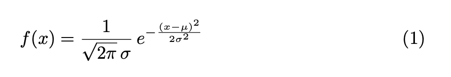
Frightening hey? even the words “probability density function” may scare the horses. I do however teach that the standard deviation is the horizontal distance between the mean and the points of inflection either side which seems to give some feeling for the curve.

Some useful properties of the normal distribution are common sense. For example,  if X has a normal distribution, then for X+10 the distribution is moved to the right by 10 units, and for 2X the distribution is spread out by a factor 2. But recently, tutoring a very good secondary school student, she thought X+10 would move the distribution left, and for 2X it would be squeezed up. She had been exposed to the formula (1) and was of course thinking that X+10 would have probability density function f(x+10), and that 2X would have f(2x). When I (hopefully) convinced her otherwise, she was concerned that the area under the graph for 2X  would no longer be 1. This is an example of where the student who knows more is more likely to be confused.

In case you are also confused, the general principle is that if X has probability density function f(x), then X+k has p.d.f. f(x-k), and kX has  (1/k)f(x/k), assuming k > 0. I’ve only ever taught this once, to some fourth year engineering students who needed to know some reliability theory. Should we teach this in Year 12? Should we even mention the formula (1)?

Switching to romantic mode …

It seems that Gauss had an unerring nose for the profound. When two Gaussian functions convolve, their offspring is … another Gaussian. Other L2 functions, those that are not Gaussian, seem to aspire to this; when they convolve their children are smoother and closer to Gaussian in shape. The Fourier spectrum of a Gaussian is a Gaussian. The Heisenberg uncertainty principle is the physical equivalent of a mathematical inequality where the extreme case is a Gaussian. Less surprising is that, in Young’s convolution inequality, the critical case is for Gaussians, and this solves a problem relating to Bonsall’s generalization of Hilbert’s famous inequality. All of this relates somehow to the unsolved mystery of the operator norm of the Laplace transform. Perhaps a taste of Gauss’s formula is warranted in secondary schools. Maybe just e^{-x^2}.


33 responses to “The Formula for a Normal Distribution”

  1. The very last sentences appear as being a 5x fast forward, but then I am not a physicist.

    Like

    1. Yes, deliberately fast. But it’s mathematics with just a passing reference to physics?

      Like

    2. I’m following the classical seminar plan for a post-graduate student: first third is to explain to the undergraduates, second third is for fellow post-graduates, and the final third for your supervisor (in my case the late E. R. Love). That third part can be faked by mentioning sufficient famous mathematicians.

      Like

      1. Thanks Tom for your reply, in particular for saying that the device was deliberate. My own comment on not being a physicist was to leave room for the possibility that the terms you used may be more familiar to them than to many mathematicians (in which I may err).

        Like

      2. Understood Christian, and well spotted.

        I did replace “Fourier transform” with “Fourier spectrum” to give a more physicsy flavour.

        Like

  2. […] Peachey has a new post on his blog: The Formula for a Normal Distribution. It is an interesting discussion of how a […]

    Like

  3. I think it’s a good idea to give students a sense of where the maths goes and show them the formula. Of course you need to make it clear that it’s not assessable, but it seems to me part of giving them a sense of the wondrous nature of maths and how it all ties together.

    The fact that things go in reverse with eg. +2 is a theme repeated in so many transformations – so very well worth spending time on.

    Like

    1. Thanks JJ. That’s one vote for teaching the formula, and also how the pdf is affected?

      Like

  4. It would be interesting to ask your very good secondary school student how they think the pdf for X would transform to give the pdf of Y = 2X -1, say.

    Applying ‘transformation of functions’ to the pdf of X gives the horizontal translation and a horizontal dilation (that is incorrect) but fails to give the vertical dilation necessary to maintain an area under the curve equal to 1. The vertical dilation has to be added ‘artificially’.

    I have seen the same misconception among many Maths Methods teachers. Any correct treatment of the transformation of a random variable is beyond the scope of the VCE Study Design.

    I think the misconception could have been reinforced by the VCAA 2022 Maths Methods Exam 2 Question 3 part (b) (iii). The rv H is transformed to 3 – H and VCAA obtains the correct answer by using ‘transformations of functions’. The method used is not valid and only gives the correct answer because there is no ‘dilation’. Many SAC 3’s have passed my way since 2022 that include such questions.

    Like

  5. Interesting. Of course the correct transformation, f(x) to (1/k)f(x/k), does retain total area 1 because of the 1/k at the front. Most problems involving transformations of normal random variables can be correctly handled, just using expectations of mean and variance, which I think is in the syllabus. So, do we need to show the pdf formula?

    Like

    1. Most problems involving transformations of normal random variables can be correctly handled, just using expectations of mean and variance, which I think is in the syllabus. So, do we need to show the pdf formula?”

      This assumes (correctly) that when X ~ Normal and X –> Y = aX + b, then Y ~ Normal. How would you prove (or at least, plausibly argue) that this is true to a Yr 12 student?

      And an inquisitive student will naturally wonder whether the above generalises to a continuous rv X that follows any distribution. (Cambridge Exercise 15D Question 5 (d) and (e) can only be done within the Study Design by assuming such a generalisation).

      Tom, you’re skirting around a very bad omission in VCE Mathematics: The omission of the cumulative distribution function (cdf). If it was part of the Study Design, finding the pdf of a linear transformation of a continuous rv is readily, correctly and naturally done. As well as many other things.

      PS – The pdf of the normal distribution is explicitly part of the Study Design, so the question of should we show the pdf formula is clearly yes.

      Like

      1. I’ll count that as a vote for including the formula, though we are not doomed to the current Study Design.

        Once we begin to justify the use of the normal distribution, the problem is where to stop. For example if independent random variables X and Y are normally distributed, should we prove that X+Y is also?

        It would be nice to see the full details of your recommended approach. But it’s difficult to post a mathematical offering with the editor here. If you want to write it up with another editor, say as a pdf or png, I will try to insert it.

        Like

      2. Once we begin to justify the use of the normal distribution, the problem is where to stop. For example if independent random variables X and Y are normally distributed, should we prove that X+Y is also?

        What proof would you propose? The current limitations of the Study Design surely suggest the answer to your question.

        Why should using the normal distribution mean that proofs of theorems such as this are required? How many theorems are used in secondary school mathematics without formal proof? What sort of secondary school curriculum would we have if everything required formal proof before it could be used?

        It’s not obvious that the sum of two normals is normal, and the result certainly doesn’t generalise: If X and Y are rv’s with distributions from the same ‘family’ then X + Y does not in general belong to the same family. So would you want to then discuss ‘stable’ distributions (of which the normal distribution is one such example). It would be nice if the Study Design for Specialist Mathematics deleted hypothesis testing and added things like the cdf and moment generating functions (the latter could be used to prove the sum of two normals result).

        As a postscript to the Y = aX + b discussion, it is not true in general that Y belongs to the same family as X. This property is only true for location-scale families of distributions (of which the normal distribution is one such example). The obvious (for a student) is often neither obvious or true.

        Like

      3. That is my point. I was implying that some theory is beyond what we can expect at this level. You seemed to be advocating for more justification of the Year 12 methods: “The omission of the cumulative distribution function (cdf). If it was part of the Study Design, finding the pdf of a linear transformation of a continuous rv is readily, correctly and naturally done. As well as many other things.

        But when I ask how far would you go, would you include adding normal variates for example, you are now implying that that is what I want. Have I misunderstood you?

        Like

      4. Adding normal variates is not in the Maths Methods Study Design, and is not needed in Maths Methods. I am not advocating for it to be in Maths Methods. It is in the Specialist Maths Study Design and is often used. The result can be used without proof. What I am saying that if hypothesis testing was deleted from Specialist Maths then other (more mathematical) things could be included which would make more proofs possible (as well as enabling the pdf of a transformed continuous rv to be correctly calculated).

        Like

      5. OK that makes sense.

        Like

  6. I get annoyed when I see the normal distributions referred to simply as a “bell shaped distribution”. The Cauchy distribution is bell-shaped, although it has no mean and no variance.

    Like

    1. The Cauchy rv is my favourite counter-example to the claim that all continuous rv’s have a mean. However, the proof that the mean does not exist is beyond the scope of VCE mathematics since it requires a careful and correct treatment of improper integrals. Calculating the mean involves integrating an odd function, and a student might naturally (and incorrectly) assume that the mean is therefore zero (implicitly using the Cauchy principle value, which is what a CAS calculator does, reinforcing the misconception). This raises another very bad omission of VCE Mathematics: Improper integrals are not included (despite the fact that they naturally arise when calculating probability, means etc. within the Study Design).

      The Cauchy distribution is what’s known as ‘fat-tailed’. It’s interesting to note that if the standard normal distribution is drawn to scale on a sheet of paper so that its ordinate at z = 6 is 1mm high, then the corresponding standard Cauchy ordinate is nearly 1.4 km high.

      An implication of the mean not existing is that if a random sample is drawn from a Cauchy distribution, then the limit of the sample mean as the sample size increases does not exist.

      Like

      1. Perhaps it should be added that if X and Y are two independent normal random variables each with zero mean, then the quotient U = X/Y has a Cauchy distribution with median equal to zero. This, perhaps, offers insight into why the mean of a Cauchy rv does not exist.

        Like

      2. I agree with you, and I like your example of comparing the graphs! IMO, students should not learn about the Normal distribution until they have a solid grounding in integral calculus – probably second year university. In spite of our shared opinion, the term “bell shaped distribution” is often used not only in school mathematics, but in many university courses in applied statistics.

        Like

      3. Indeed Terry. We are straying from the original focus of secondary school mathematics, but what is say a university lecturer to do if teaching applied statistics to a class of innumerate psychology students. A long gone colleague of mine used the “shut up and follow the recipe” approach. But even his psychology students wanted some glimmer of understanding.

        Like

  7. I don’t have a good answer to your question. As for teaching students of psychology, it is also annoying to me that it is expected that the students get a grip on factor analysis without knowing anything about matrices.

    Like

  8. Could you clarify what the “unsolved mystery of the operator norm of the Laplace transform” is?

    Like

    1. In my mind, the question is to put a number on it:

      https://www.tandfonline.com/doi/full/10.1080/10652469.2022.2026351

      My feeling is that a generalization of the inequality for the Heisenberg uncertainty principle will solve it.

      Like

      1. Oh interesting, thanks. I’d known the L2 result but didn’t ever consider higher norms. Do you have reason to believe there’s a nice form for general p?

        Like

      2. Well I managed to derive an integral equation for the maximizer, but then managed to prove that the equation has no solutions.

        Like

      3. It must be an important problem, one of the few unsolved ones mentioned by Hardy, Littlewood and Polya, Inequalities, Theorem 352. Back in the 70s, Arthur Erdelyi had me working on a related problem.

        Like

  9. Hi Tom,

    Can I have a copy of your short note? It sounds interesting, and I don’t have access to the publisher version…

    cheers

    Glen

    Like

    1. Hi Glen

      You are very welcome. It’s attached. Tom

      Like

      1. Hi Tom! I’m probably tragically inept at using this webpage, but I somehow can’t see where exactly it is attached….

        Like

      2. It’s not you, it was my stupidity. Short of exchanging emails, I suggest the following. Go to https://www.researchgate.net/search.Search.html?query=&type=publication

        ( You don’t need to sign up to ResearchGate.) In the search field enter the paper name.

        A Note on the Operator Norm of the Laplace Transformation

        It hopefully will let you download the paper.

        I’m guessing the paper will be a disappointment to you. The result is an outlandish formula, and the method of getting it is just an application of a more general result. And it’s still not the actual norm. Well, Hardy was pessimistic about getting a full solution.

        Liked by 1 person

  10. Hi Tom!

    I went there and found your paper after searching, but not a download of it. I clicked “request full text”. I hope that you may be able to provide one…?

    Cheers!

    Like

    1. Damn. When I looked it let me download, but must have remembered that I was the supplier. I have now sent a copy via the ResearchGate mechanism – I hope.

      On a more general note, there was a time when one could walk into a library and peruse the journals. It seems you have the same problem as me; access is now online and outsiders to the system can no longer avail this.

      Like

Leave a reply to Mystery Person Cancel reply